Examples

The following examples detail the simulation of QVAs for unconstrained and constrained combinatorial optimisation problems.

The examples are size so they may be easily ran on most personal computers. The examples must be ran using the mpiexec or mpirun launchers. For example, to run the QAOA maxcut example located in examples/maxcut on a system with 4 CPU cores:

mpiexec -N 4 python3 maxcut.py

Maxcut

The max-cut problem seeks to partition the vertices of a graph such that a maximum number of neighbouring nodes are assigned to two disjoint sets [FGG14]. A quantum encoding of the max-cut problem is a bijective mapping of the vertices of a graph \(G\) to \(n\) qubits, with the set membership indicated by the corresponding qubit state. For example, a two vertex graph with vertices \({\left\{0,1\right\}}\) has a solution space that is completely represented by an equal superposition over a two-qubit system: \({\left\{{\left\{0,1\right\}}\right\}} \rightarrow {\lvert 00\rangle}\), \({\left\{{\left\{0\right\}},{\left\{1\right\}}\right\}} \rightarrow {\lvert 01\rangle}\), \({\left\{{\left\{0\right\}},{\left\{1\right\}}\right\}} \rightarrow {\lvert 10\rangle}\) and \({\left\{{\left\{0,1\right\}}\right\}} \rightarrow {\lvert 11\rangle}\).

The cost function is then implemented as

(1)\[ {C(s)} = \sum_{E(i,j)\in G} \frac{1}{2}\left( \mathbb{I} + Z_iZ_j\right),\]

where \(Z_i\) is a Pauli Z gate acting on the \(i^\text{th}\) qubit, \(E(i,j)\) is an edge in \(G\) connecting vertex \(i\) to vertex \(j\), and \(Z_iZ_j\) has eigenvalue \(1\) if qubits \(i\) and \(j\) are in the same state or \(-1\) otherwise.

QAOA (Serial Quality Function)

• examples/maxcut/maxcut.py

Here the QAOA is applied to the max-cut problem for the graph shown below. The predefined Ansatz subclass qaoa forms the basis of the simulation.

System Message: WARNING/2 (/home/runner/work/QuOp_MPI/QuOp_MPI/docs/source/examples.rst, line 55)

Cannot scale image! Could not get size from "_static/maxcut_graph.png": Requires Python Imaging Library.

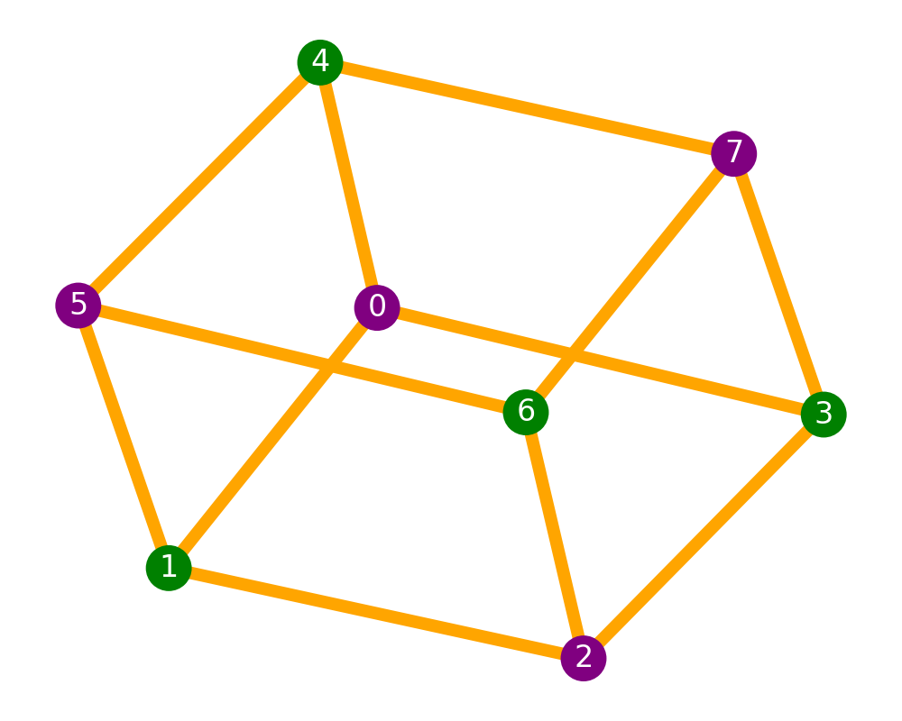
Graph for the example maxcut problem. The green and purple vertices indicate one of two optimal vertex partitioning.

To generate the graph we use the external package networkx. And define the cost function as a Python function using the I and Z functions from toolkit, we are able to directly implement (1).

from quop_mpi.algorithm.combinatorial import qaoa, serial
from quop_mpi.toolkit import I, Z
import networkx as nx

Graph = nx.circular_ladder_graph(4)

vertices = len(Graph.nodes)
system_size = 2 ** vertices

G = nx.to_scipy_sparse_array(Graph)

def maxcut_qualities(G):
    C = 0
    for i in range(G.shape[0]):
        for j in range(G.shape[0]):
            if G[i, j] != 0:
                C += 0.5 * (I(vertices) - (Z(i, vertices) @ Z(j, vertices)))
    return -C.diagonal()

A qaoa instance is instantiated. and the \(\text{diag}(\hat{Q})\) (the solution qualities) is defined via the set_qualities() method. For this, we pass the serial() Observables Function along with a dictionary containing maxcut qualities and its arguments. The serial function assists with memory-efficient simulation, by calling the maxcut_qualities at the root MPI process and distributing its output over Ansatz subcommunicator. The ansatz depth (\(D=2\)) is defined via the set_depth().

alg = qaoa(system_size)
alg.set_qualities(serial, {'args':[maxcut_qualities, G]})
alg.set_depth(2)

Now that the qaoa instance is fully specified, simulation of the algorithm (see QAOA) proceeds via execute(). By calling execute without specifying the initial variational parameters we use the default Parameter Functions, which generates variational parameters from a uniform distribution over \((0 \pi, 2\pi]\).

alg.execute()

Finally, the optimiser result is displayed using print_result() and the simulation results are saved to the HDF5 file ‘maxcut.h5’ under the ‘depth 2’ group.

alg.print_result()
alg.save("maxcut", "depth 2", "w")

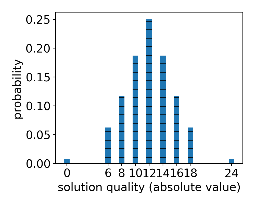
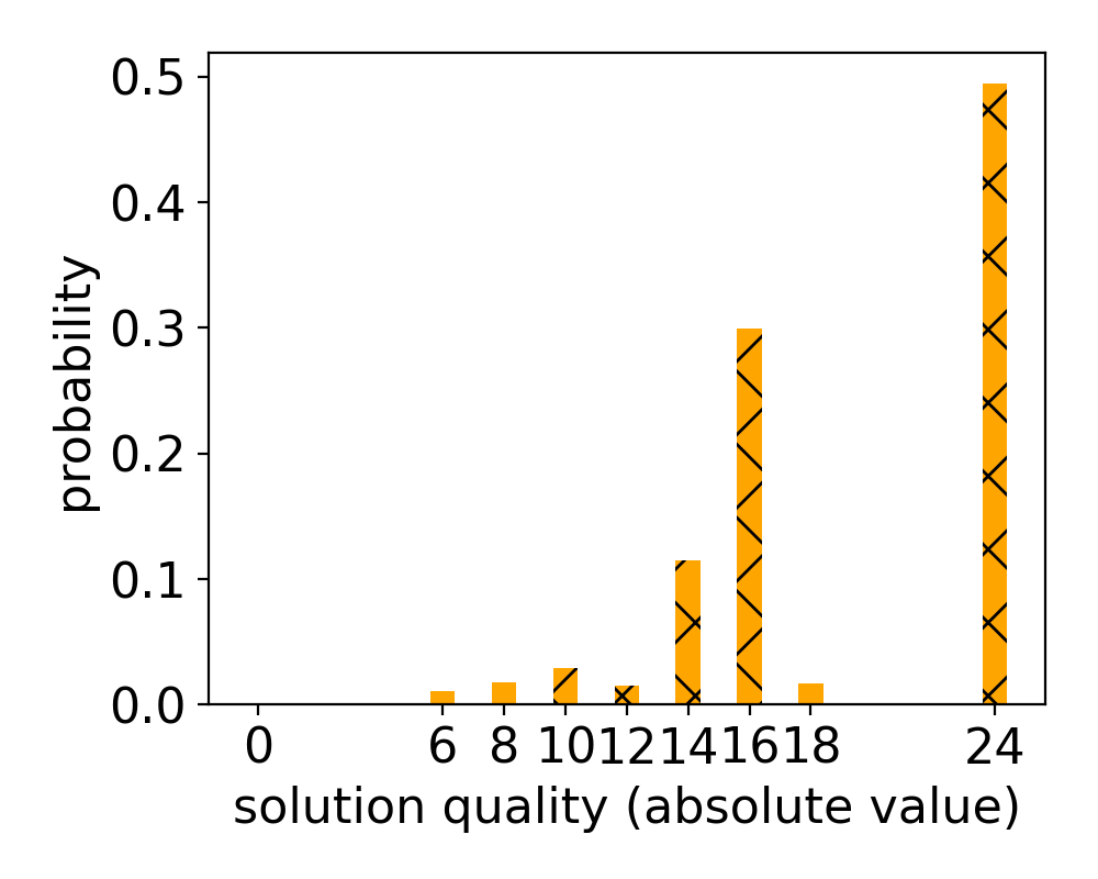
The figure below illustrates the initial and final probability distributions with respect of the unique values of \(q_i\) (see observables). After application of the QAOA to the initial superposition, probability density is concentrated at high-quality solutions with the optimal solution having the highest probability of measurement.

The starting probability of the maxcut problem solution qualities (left) and the equivalent probability distribution after execution of the QAOA.

QAOA (Parallel Observables Function)

• examples/maxcut/maxcut_parallel_qualities.py

Here we consider a variation on the above QAOA example, whereby the cost function given in (1) is computed via a user-defined Operator Function. As, previously we require qaoa and networkx. We also import NumPy.

from quop_mpi.algorithm.combinatorial import qaoa
import numpy as np
import networkx as nx

The graph is generated using networkx and the system size computed from the number of graph nodes.

Graph = nx.circular_ladder_graph(4)
nodes = len(Graph.nodes)
system_size = 2 ** nodes
G = nx.to_scipy_sparse_array(Graph)

An Operator Function is a QuOp Function that returns the matrix operator of a unitary. The QAOA phase-shift unitary has a diagonal matrix operator that contains the solution qualities (which also define the QAOA observables). An Operator Function for the computation of the solution qualities must return a 1-D real array containing local_i elements with global index offset local_i_offset. We are able to compute the maxcut solution qualities in parallel as computation of the quality for any specific solution is independent of the global solution space.

def parallel_maxcut_qualities(local_i, local_i_offset, G):

    n_qubits = G.shape[0]
    qualities = np.zeros(local_i, dtype=np.float64)
    start = local_i_offset
    finish = local_i_offset + local_i

    for i in range(start, finish):
        bit_string = np.binary_repr(i, width=n_qubits)
        for j, bj in enumerate(bit_string):
            for k, bk in enumerate(bit_string):
                if G[j, k] != 0 and int(bj) != int(bk):
                    qualities[i - local_i_offset] -= 1
    return qualities

The parallel_maxcut_qualities Operator Function is passed to set_qualities(). As, its local_i and local_i_offset arguments are attributes of the Ansatz class, they will be passed to the function automatically. The G argument is specified as an additional positional argument in a corresponding FunctionDict.

alg = qaoa(system_size)
alg.set_qualities(parallel_maxcut_qualities, {'args':[G]})
alg.set_depth(2)
alg.execute()
alg.print_result()
alg.save("maxcut_parallel_qualities", "depth 2", "w")

Ex-QAOA

• examples/maxcut_extended/maxcut_extended.py

Here we address the maxcut problem defined above using the Extended-QAOA. We will do this by implementing a QVA using the Ansatz base-class, the diagonal propagator to simulate the action of the Ex-QAOA phase-shift unitary and the sparse propagator to simulate the action of the Ex-QAOA mixing unitary. The serial() Observables Function will be used to interface a serial Python function for computation of the maxcut solution qualities (see (1)) with QuOp_MPI. Finally, the Z() Pauli operator function from toolkit will be used to efficiently implement the parameterised Ex-QAOA phase-shift unitary matrix operator.

import numpy as np
import networkx as nx
from quop_mpi import Ansatz
from quop_mpi.propagator import diagonal, sparse
from quop_mpi.observable import serial
from quop_mpi.toolkit import Z

The problem graph is generated using networkx and the system size computed from the number of graph vertices.

vertices = len(Graph.nodes)
system_size = 2 ** vertices
G = nx.to_scipy_sparse_array(Graph)
n_edges = 2 * Graph.number_of_edges()

The maxcut_terms functions implements the Ex-QAOA phase-shift unitary by returning a list of 1-D arrays that correspond to the non-identity Pauli terms in the problem cost function (see qaoa-cost)). Each of these terms will associated with a phase-shift unitary with independently parameterised operator parameters.

def maxcut_terms(G):
    vertices = G.shape[0]
    terms = []
    for i in range(G.shape[0]):
        for j in range(G.shape[0]):
            if G[i, j] != 0:
                term = Z(i, vertices) @ Z(j, vertices)
                terms.append(-0.5 * (1 - term.diagonal()))
    return terms

Due to these extra degrees of freedom, the the Ex-QAOA phase-shift unitary does not contain the QVA observables. As such, the observables are independently computed via the max_qualities function, which sums the output of maxcut_terms returning the solution qualities as defined in (1).

def maxcut_qualities(G):
    return np.sum(maxcut_terms(G), axis = 0)

The phase-shift unitary UQ is implemented via an instance of the diagonal unitary class. The unitary_n_params specifies the number of unitary parameters associated with the unitary.

UQ = diagonal.unitary(
    diagonal.operator.serial,
    operator_dict={"args": [maxcut_terms, G]},
    unitary_n_params=n_edges
)

UW = sparse.unitary(sparse.operator.hypercube)

The ansatz unitary is specified by passing [UQ, UW] to set_unitaries(). Simulation then proceeds with the default quop_mpi.Ansatz `:term:`initial state (an equal superposition).

alg = Ansatz(system_size)
alg.set_unitaries([UQ, UW])
alg.set_observables(serial, {"args": [maxcut_qualities, G]})
alg.set_depth(2)
alg.execute()
alg.print_result()
alg.save("maxcut_extended", "depth 2", "w")

System Message: WARNING/2 (/home/runner/work/QuOp_MPI/QuOp_MPI/docs/source/examples.rst, line 178)

Cannot scale image! Could not get size from "_static/maxcut_extended_qaoa_probabilities.png": Requires Python Imaging Library.

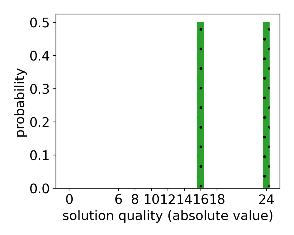
Probability distribution of the maxcut problem solution qualities after execution of the Ex-QAOA.

Portfolio Rebalancing

To explore the case of constrained optimisation using the QWOA and the QAOAz we will consider the problem of portfolio re-balancing. For each asset in a portfolio of size \(M\), an investor must choose one of the following positions:

1. Short position: buying and selling an asset with the expectation that it will drop in value.

2. Long position: buying and holding the asset with the expectation that it will rise in value.

3. No position: taking neither the long or short position.

A quantum encoding of the possible solutions uses two qubits per asset.

1. \({\lvert 01\rangle} \rightarrow \text{short position}\)

2. \({\lvert 10\rangle} \rightarrow \text{long position}\)

3. \({\lvert 00\rangle}\) or \({\lvert 11\rangle} \rightarrow \text{no position}\)

The discrete mean-variance Markowitz model provides a means of evaluating the quality associated with a given combination of positions. It can be expressed through minimisation of the cost function,

\[{C(s)} = \omega \sum_{i,j = 1}^{M} \sigma_{ij}Z_iZ_j - (1 - \omega) \sum_{i = 1}^{M} r_iZ_i,\]

subject to the constraint,

\[{\chi_{\text{asset}}(s)} = \sum_{i = 1}^{M} z_i.\]

In this formulation, the Pauli-Z gates \(Z_i\) encode a particular portfolio where, for each asset, eigenvalue \(z_i \in {\left\{1,-1,0\right\}}\) represents a choice of long, short or no position. Associated with each asset is the expected return \(r_i\) and covariance \(\sigma_{ij}\) between assets \(i\) and \(j\); which are calculated using historical data. The risk parameter, \(\omega\), weights consideration of \(r_i\) and \(\sigma_{ij}\) such that as \(\omega \rightarrow 0\) the optimal portfolio is one providing maximum returns. In contrast, as \(\omega \rightarrow 1\), the optimal portfolio is the one that minimises risk. The constraint \({\chi_{\text{asset}}(s)}\) works to maintain the relative net position with respect to a pre-existing portfolio [SMMW21].

In the following examples, we demonstrate the application of the QWOA and QAOAz to a small ‘portfolio’ consisting of four assets taken from the ASX 100, under the constraint \({\chi_{\text{asset}}(s)} = 2\).

QAOAz

• examples/portfolio_rebalancing/qaoaz_portfolio.py

• examples/portfolio_rebalancing/qaoaz_qualities.py

A QAOAz approach to the portfolio optimisation problem uses two parity mixers that act on the short and long qubits, respectively, such that the \({\mathcal{S}}\) is partitioned into subgraphs of the same \({\chi_{\text{asset}}(s)}\) value. For this example, we are considering four assets so the two parity mixers act on separate subspaces of \(\mathcal{H}\) as shown below:

System Message: WARNING/2 (/home/runner/work/QuOp_MPI/QuOp_MPI/docs/source/examples.rst, line 254)

Cannot scale image! Could not get size from "_static/portfolio_parity.png": Requires Python Imaging Library.

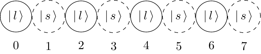
Where \({\lvert l\rangle}\) denotes a ‘long’ qubit, \({\lvert s\rangle}\) denotes a ‘short’ qubit, and the numbering indicates the global index of each qubit.

To constrain probability amplitude to \({\mathcal{S}^\prime}\), \({{\lvert\psi_0\rangle}_\text{QAOAz}}\) is prepared as

(2)\[{{\lvert\psi_0\rangle}_\text{QAOAz}} = {\lvert 01\rangle}^{\otimes A}\left( \frac{1}{\sqrt{2}}({\lvert 00\rangle} + {\lvert 11\rangle})^{2N-A} \right),\]

where \(A\) is the desired value of \({\chi_{\text{asset}}(s)}\). This creates a (non-equal) superposition of states across all qubit subgraphs with a net parity of \(A\).

Here we implement the QAOAz using the Ansatz base-class, the diagonal propagator module, the sparse propagator module and the quop_mpi.state module. The string(), X(), Y, kron() and kron_power() functions from toolkit are imported to assist with the definition of functions for the QAOAz parity mixing unitary and initial state (see (2)). The qaoaz_portfolio function imported from qaoaz_qualities (examples/portfolio_rebalancing/qaoaz_qualities.py) is an Operator Function that computes the solution qualities based on adjusted close price historical data obtained from Yahoo Finance.

from numpy import sqrt
from quop_mpi import Ansatz, state
from quop_mpi.propagator import diagonal, sparse
from quop_mpi.toolkit import kron, kron_power
from quop_mpi.toolkit import string, X, Y
from qaoaz_qualities import qaoaz_portfolio

The parity_ring, parity_mixer and mixer functions generate the QAOAz mixing unitary operator as a CSR sparse matrix.

def parity_ring(i, j, n_qubits):
    parity = X(i, n_qubits) @ X(j, n_qubits) + Y(i, n_qubits) @ Y(j, n_qubits)
    return parity

def parity_mixer(qubits, n_qubits):

    odd = 0
    even = 0
    n_subset = len(qubits)

    for i in range(n_subset - 1):
        if i % 2 != 0:
            odd += parity_ring(qubits[i], qubits[(i + 1) % n_subset], n_qubits)
        elif i % 2 == 0:
            even += parity_ring(qubits[i], qubits[(i + 1) % n_subset], n_qubits)

    mixer = [odd, even]

    if len(qubits) % 2 != 0:
        last = parity_ring(qubits[-1], qubits[1], n_qubits)
        mixer.append(last)

    return mixer


def mixer(n_qubits):
    short_qubits = [i for i in range(0, n_qubits, 2)]
    long_qubits = [i for i in range(1, n_qubits, 2)]
    short_mixer = parity_mixer(short_qubits, n_qubits)
    long_mixer = parity_mixer(long_qubits, n_qubits)
    return short_mixer + long_mixer

Next, the parity_state function implements (2),

def parity_state(n_qubits, D):
    M = n_qubits // 2
    term_1 = kron_power(string("01"), D)
    term_2 = kron_power(1 / sqrt(2) * (string("11") + string("00")), M - D)
    return kron([term_1, term_2])

and the system size is calculated from the number of qubits required to represent 4 assets.

n_qubits = 8
system_size = 2 ** n_qubits

The phase-shift and mixing unitaries are defined via instances of the diagonal and sparse unitary classes.

UQ = diagonal.unitary(diagonal.operator.observables)

UW = sparse.unitary(
    sparse.operator.serial,
    operator_dict={"args": [mixer, n_qubits]}
)

The ansatz unitary is defined by passing [UQ, UW] to set_unitaries() and the observables defined by passing the index of UQ to set_observables().

alg = Ansatz(system_size)
alg.set_unitaries([UQ, UW])
alg.set_observables(qaoaz_portfolio)
alg.set_initial_state(state.serial, {"args": [parity_state, n_qubits, 2]})

To assist with the analysis of QVA performance, QuOp supports the recording of important simulation metrics in a log file. The set_log() method specifies the recording of the system size, ansatz depth, optimised objective function value, norm of the final state, in-program simulation time, MPI communicator size, number of objective function evaluates and the success status of the classical optimiser to qaoaz_portfolio.csv for each simulation instance.

alg.set_log("qaoaz_portfolio_log", "qaoaz", action="w")

We are often interested in evaluating the performance of a QVA as a function of the ansatz depth. For this, we use benchmark(), which will carry out a sequence of calls to execute() over the ansatz depth range of 1 to 5, with 3 repeats per ansatz depth.

alg.benchmark(
    range(1, 6), 3, param_persist=True, filename="qaoaz_portfolio", save_action="w"
)

QWOA

• examples/portfolio_rebalancing/qwoa_portfolio.py

• examples/portfolio_rebalancing/qwoa_qualities.py

Here we address the portfolio optimisation problem using the QWOA, which carries out a quantum search over the subspace of valid solutions. For this we will use the predefined qwoa algorithm and the csv() Operator Function.

from quop_mpi.algorithm.combinatorial import qwoa, csv

The system state is set equal to the number of valid solutions (31),

system_size = 31
alg = qwoa(system_size)

and the observables and phase-shift unitary matrix operator specified by set_qualities(). The 'args' and 'kwargs' items in the corresponding FunctionDict are passed to the pandas read_csv function. The solution quality values are retrieved from qwoa_qualities.csv, which have been precomputed using examples/portfolio_rebalancing/qwoa_qualities.py.

alg.set_qualities(
    csv, 
    {
        "args": ["qwoa_qualities.csv"],
        "kwargs": {'usecols':[1], 'header':None}
    }
    )

Finally, the logging of simulation data is specified and the algorithm simulated from ansatz depths 1 to 6 with 3 repeats per ansatz depth using benchmark().

alg.set_log("qwoa_portfolio_log", "qwoa", action="w")
alg.benchmark(
    range(1, 6),
    3,
    param_persist=True,
    filename="qwoa_portfolio",
    save_action="w"
)

System Message: WARNING/2 (/home/runner/work/QuOp_MPI/QuOp_MPI/docs/source/examples.rst, line 343)

Cannot scale image! Could not get size from "_static/portfolio_rebalancing.png": Requires Python Imaging Library.

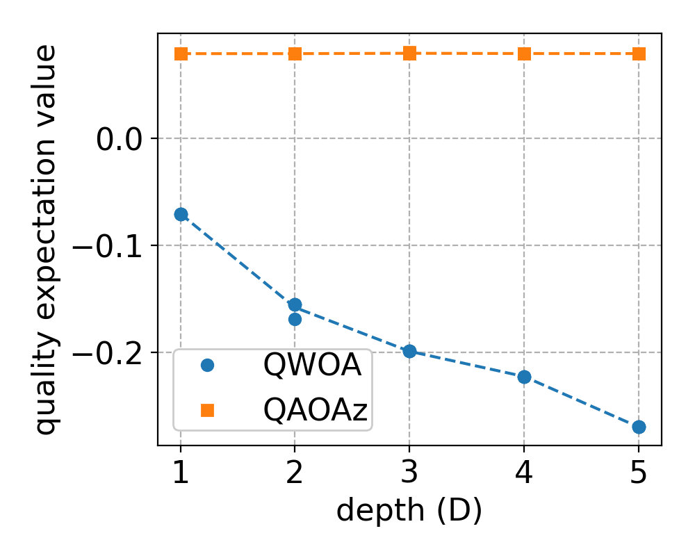
Final objective function value achieved by the QAOAz and the QWOA for a portfolio optimisation problem with 4 assets from ansatz depths 1 to 5. each point depicts the average of three repeats.