Theoretical Background
The following sections contain excerpts from:
Matwiejew, E. & Wang, J. B. QuOp_MPI: A framework for parallel simulation of quantum variational algorithms. Journal of Computational Science 62, 101711 (2022). DOI:10.1016/j.jocs.2022.101711
Matwiejew, E., Pye J. & Wang J. B. Quantum Optimisation for Continuous Multivariable Functions by a Structured Search. arXiv:2210.06227 (2022). arXiv
Combinatorial Optimisation
Quantum Variational Algorithms
For a quantum system of size \(N = 2^n\), where integer \(n\) is a number of qubits with basis states \({\left\{{\lvert 0\rangle} = \begin{pmatrix} 0 \\ 1 \end{pmatrix},{\lvert 1\rangle} = \begin{pmatrix} 1 \\ 0 \end{pmatrix}\right\}}\), QuOp_MPI defines a generalised QVA as
where \({{\lvert\psi_0\rangle}} \in \mathbb{C}^{N}\) is an initial quantum state with basis states \({\left\{{\lvert i\rangle}\right\}}_{i=0,...,N-1}\), \({\hat{U}_{}} \in \mathbb{C}^{N \times N}\) is the ansatz unitary , integer \(p \geq 0\) specifies the number of applications of \({\hat{U}_{}}\) to \({{\lvert\psi_0\rangle}}\) (the ‘depth’) and \(\bm{\theta}= \{ \theta_i \in \mathbb{R} \}\) is an ordered set of classically tunable values that parameterise \({\hat{U}_{}}\). The ansatz unitary \({\hat{U}_{}}\) and initial quantum state \({{\lvert\psi_0\rangle}}\) together define a specific QVA.
A Quantum Variational Algorithm is executed by repeatedly preparing \({{\lvert\bm{\theta}\rangle}}\) and measuring the expectation value
where \(\hat{Q}\in \mathbb{R}^{N \times N}\) is a diagonal matrix operator with entries \(\text{diag}(\hat{Q}) = q_i\) that specify the ‘quality’ associated with quantum state \({\lvert i\rangle}\). The variational parameters \(\bm{\theta}\) are updated using a classical optimiser with the objective being minimisation of \(f\).
The ansatz operator \({\hat{U}_{}}\) specifies a sequence of alternating unitaries. This can include phase-shifts
where \(\hat{O} = \sum_{i=0}^{N-1} o_i {\lvert i\rangle}{\langle i\rvert}\) is a diagonal phase-shift matrix operator, \(\gamma \in \bm{\theta}\) and \(\hat{U}_\text{phase}\) applies a phase-shift proportional to \(o_i\), as well as mixing-unitaries
where \(t \in \bm{\theta}\) is non-negative and \(\hat{W} = \sum_{{i,j} = 0}^{n-1}w_{ij}{\lvert j\rangle}{\langle i\rvert}\) is a mixing matrix operator in which non-diagonal entries specify coupling between states \({\lvert i\rangle}\) and \({\lvert j\rangle}\). Mixing-unitaries \(\hat{U}_\text{mix}\) drive the transfer of probability amplitude between quantum states, during which encoded phase differences contribute to constructive and destructive interference.
Phase-shift operators \(\hat{O}\) and mixing operators \(\hat{W}\) may also be parameterised by \(\bm{\theta}\). As these operators are time-independent Hamiltonians of the time-evolution operator, changes to the corresponding \(\theta_i\) alter the element-wise magnitudes or structure of the matrix exponent before preparation of \({{\lvert\bm{\theta}\rangle}}\).
Typically, the ansatz unitary \({\hat{U}_{}}\) is applied \(p\) times to \({{\lvert\psi_0\rangle}}\) with each repetition parameterised by subset \(\theta \subseteq \bm{\theta}\). Doing so increases the potential for constructive and destructive inference to concentrate probability amplitude at high-quality solutions; at the expense of classical optimisation over a larger parameter space and a deeper quantum circuit. In practice, a QVA must balance the improved convergence afforded by increases to \(p\) against the ability of the quantum hardware to maintain coherence over a longer sequence of quantum operations.
The following sections introduce four distinct QVAs for solving constrained and unconstrained COPs. We summarise here the following notational conventions for a given QVA:
\(n\): the number of qubits.
\({{\lvert\psi_0\rangle}}\): the initial quantum state vector.
\({\hat{U}_{}}\): a sequence of phase-shift and mixing operators.
\({\lvert\psi\rangle}\): \({{\lvert\psi_0\rangle}}\) after \(p \geq 0\) applications of \({\hat{U}_{}}\).
\({{\lvert\bm{\theta}\rangle}}\): \({{\lvert\psi_0\rangle}}\) after \(p \geq 1\) applications of \({\hat{U}_{}}\).
\(\bm{\theta}\): classically tunable variables parameterising \({\hat{U}_{}}\) with starting values \(\bm{\theta}_0\) and optimised values \(\bm{\theta}_f\).
\(f\): the ansatz objective function.
Combinatorial Optimisation with QVAs
Combinatorial optimisation problems seek optimal solutions \({\Bar{s}}\) of the form,
where the problem cost-function \({C(s)}\) maps a solution \(s\) from an ordered set of problem solutions \(\mathcal{S} = {\left\{s_i\right\}}\) to \(\mathbb{R}\), \(s\) is a \(k\)-permutation of discrete elements from a finite set \({\bm{\zeta}}\) and
is the problem-specific valid solution space where
denotes any constraints on \({\Bar{s}}\) and \(\bm{a} = {\left\{a_i\right\}}\) defines the constraints.
Problems of this type are often difficult to solve as \({\mathcal{S}}\) grows factorially with \({\left|{\bm{\zeta}}\right|}\) and, in general, lacks identifiable structure. For this reason, heuristic and metaheuristic algorithms are often used to find solutions that satisfy the relaxed condition of \({C({\Bar{s}})}\) being a ‘sufficiently low’ local minimum.
To apply a quantum variational algorithm to a given combinatorial optimisation problem, an injective map is defined between \({\mathcal{S}}\) and \(\mathcal{H}\) with the cost-function values forming the diagonal of the quality operator \(\text{diag}(\hat{Q})= {C(s_i)}\). For example, a problem with four solutions, \(\mathcal{S} = \{s_0, s_1, s_2, s_3\}\), maps to a two-qubit system as
where \(\text{diag}(\hat{Q})= \Big(C(s_0),C(s_1),C(s_2),C(s_3)\Big)\).
For a combinatorial optimisation problem to be efficiently solvable by a QVA, it must satisfy three conditions:
The number of solutions \({\left|{\mathcal{S}}\right|}\) must be efficiently computable in order to establish a bound on the size of the required Hilbert space \(\mathcal{H}\).
For all solutions \(s\), \({C(s)}\) must be computable in polynomial time .
For all solutions \(s\), \({C(s)}\) must be polynomially bounded with respect to \({\left|{\mathcal{S}}\right|}\).
Conditions one and two ensure that the objective function (2) is efficiently computable as classical computation of \({C(s)}\) is required to compute \(f\) and boundedness in \({C(s)}\) ensures that the number of measurements required to accurately compute \(f\) does not grow exponentially with \({\left|{\mathcal{S}^\prime}\right|}\) [CKST99]. These conditions constrain the application of QVAs to polynomially bounded (PB) COPs in the non-deterministic polynomial-time optimisation problem (NPO) complexity class (together denoted as NPO-PB) [CKST99].
Unconstrained Optimisation
For the case of unconstrained optimisation, the valid solution space \({\mathcal{S}^\prime}\) is equivalent to \({\mathcal{S}}\). For these COPs a quantum encoding of \({C(s)}\) is equivalent to the bijective map \({\mathcal{S}}\rightarrow \mathcal{H}\).
QAOA
The Quantum Approximate Optimisation Algorithm is comprised of two alternating unitaries. Firstly the phase-shift-unitary
and, secondly, the mixing operator
where \(\hat{W}_\text{X} = X^{\otimes N}\) and \(X\) is the Pauli-\(X\) (or quantum NOT) gate. The mixing operator \(\hat{W}_\text{X}\) induces a coupling topology that is equivalent to an \(n\)-dimension hypercube graph, as shown in Fig. hypercube-mixer.
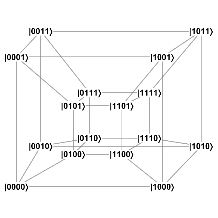
Fig. 1 Coupling topology of \(W_\text{X}\) in the QAOA for \({\left|{\mathcal{S}}\right|} = 16\) (\(n\) = 4).
The initial state \({{\lvert\psi_0\rangle}_\text{QAOA}}\) is prepared as an equal superposition over \(\mathcal{H}\),
The final quantum state is then
where \(\bm{\theta}= \{\gamma_i, t_i \}\) and \({\left|\bm{\theta}\right|} = 2p\) [FGG14].
Extended-QAOA
A variation of the QAOA, ‘extended-QAOA’ (ex-QAOA), utilises a sequence of phase-shift unitaries,
where \(\Sigma_j\) are non-identity terms in a Pauli-gate decomposition of \(\hat{Q}\) and \({\left|\Sigma\right|}\) is the number of non-identity terms [GS17]. This increases the number of variational parameters to \({\left|\bm{\theta}\right|} = (1 + {\left|\Sigma\right|})p\) with the intent of achieving a higher degree of convergence to optimal solutions at a lower circuit depth.
The final state of ex-QAOA is
where \({\lvert+\rangle}\) and \(\hat{U}_X\) are defined as in (6) and (7), and \(\bm{\theta}= {\left\{\gamma_{ij}, t_i\right\}}\).
Constrained Optimisation
Constrained optimisation problems seek valid solutions \({s^\prime}\) from a subset of \({\mathcal{S}}\) as defined by constraints \({\bm{\chi}}\). Encoding of the solution constraints \({\bm{\chi}}\) is achieved by restricting the action of the mixing-unitaries \({\hat{U}_{\text{mix}}}\) and initialising \({{\lvert\psi_0\rangle}}\) over a subspace of \(\mathcal{H}\).
QAOAz
The Quantum Alternating Operator Ansatz was developed to solve problems for which \({\bm{\chi}}\) creates a correspondence between \({\mathcal{S}^\prime}\) and quantum states of equal parity – states with the same number of \({\lvert 1\rangle}\) states. This algorithm consists of the phase-shift-unitary defined in (5), followed by a sequence of three \({\hat{U}_{\text{mix}}}\) with mixing operators
which together form the parity-conserving mixing operator
that mixes probability amplitude between subgraphs of equal parity as illustrated in Fig. parity-mixer.
By initialising \({{\lvert\psi_0\rangle}_\text{QAOAz}}\) in a quantum state that satisfies the parity constraint, probability amplitude is constrained to \({\mathcal{S}^\prime}\).
The state evolution of the QAOAz is
where \({{\lvert\psi_0\rangle}_\text{QAOAz}}\) is an initial state satisfying the parity constraint [HWOGorman+19].
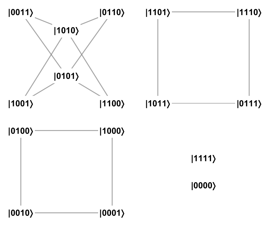
Fig. 2 Coupling topology of \(\hat{W}\) for the QAOAz (\(n = 4\)). Note that \(\mathcal{H}\) is partitioned into subgraphs of equal state parity.
QWOA
The Quantum Walk-assisted Optimisation Algorithm implements \({\bm{\chi}}\) given the existence of an efficient indexing algorithm for all \(s\in\ {\mathcal{S}^\prime}\). Under this condition, the QWOA implements an indexing unitary
where \({U^{\dag}_{\#}}\) maps states corresponding to valid solutions \({\lvert{s^\prime}\rangle}\) to indexed states \({\lvert\text{id}_{{\bm{\chi}}}(i)\rangle}\). By preparing \({{\lvert\psi_0\rangle}_\text{QWOA}}\) as an equal superposition over \({\lvert\text{id}_{{\bm{\chi}}}(i)\rangle}\)
probability amplitude is restricted to the subspace of indexed states.
The indexing unitary \({U^{\dag}_{\#}}\) and its conjugate unindexing unitary \(\hat{U}_\#\) occur either side of a mixing-unitary that acts on \({\lvert\text{id}_{{\bm{\chi}}}(i)\rangle}\):
Where efficiency in the implementation of \({U^{\dag}_{\#}}\) dictates that \(\hat{W}_\text{QWOA}\) is circulant. Most commonly, \(\hat{W}_\text{QWOA}\) is chosen to be the adjacency matrix of the complete graph as it produces a maximal and unbiased coupling over \({\lvert{\mathcal{S}^\prime}\rangle}\) (see Fig. complete-mixer).
The state evolution of the QWOA is
where \(\bm{\theta}= {\left\{\gamma_i, t_i\right\}}\) and there are \({\left|\bm{\theta}\right|} = 2p\) variational parameters [MW19b, MW20].
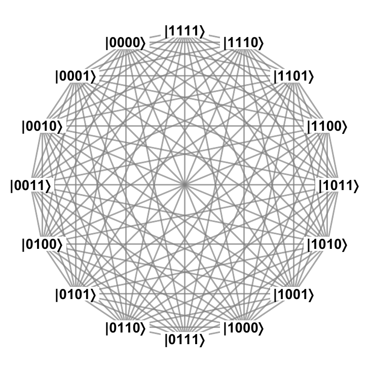
Fig. 3 A complete graph mixer, in QWOA with couples all valid solutions in the solution space.
Multivariable Optimisation
The Continuous Multivariable Optimisation Problem
For a continuous function \(f: X \rightarrow Y\), where \(X \subset \mathbb{R}^D\) and \(Y \subset \mathbb{R}\), continuous-variable optimisation seeks \({\bm{x}^*} = (x_0, ..., x_{D-1}) \in X\) satisfying,
where \(f_\text{min}\) is the global minimum of \(f\) and \(\epsilon > 0\) defines a region of accepted \(\bm{x}\) near \(f_\text{min}\).
An encoding of the optimisation problem in a system of qubits consists of evaluating \(f\) on a grid of \(K = N^D\) points. In each dimension \(d\), the coordinate is discretised as \(x_{d,n_d} = x_{d,0} + n_d \Delta x_d\), with minimum value \(x_{d,0}\), grid spacing \(\Delta x_d\), and \(n_d = 0, \dots, N-1\). The complete solution space of discretised coordinates \(\bm{x}_k\) is then represented using \(\mathcal{O}(\log K)\) qubits by states \(\ket{k} \equiv \ket{x_{D-1,n_{D-1}},x_{D-2,n_{D-2}}, \dots, x_{0,n_0}}\), where \(k = 0, \dots, N^D-1\) is a vectorised index for the set \((n_0, \dots, n_{D-2}, n_{D-1}) \in \{ 0, \dots, N-1 \}^D\). For optimisation over this discrete space, we denote the global minimum as \({\bm{x}^*} \equiv \text{argmin}_{k} f(\bm{x}_k)\).
QVAs for Optimisation of Continuous Multivariable Functions
Here we consider QVAs of the form
where the positive integer \(p\) is a fixed number of ansatz iterations, \(\hat{U}\) is the ansatz unitary, \(t_i\) and \(\gamma_i\) are real-valued variational parameters and,
unless otherwise specified. The ansatz unitary consists of the so-called alternating phase-shift, \(\hat{U}_Q\), and mixing, \(\hat{U}_W\), unitaries,
The first of these,
applies a phase-shift proportional to
where \(f_k \equiv f(\bm{x}_k)\). The second unitary, \(\hat{U}_W\), conforms to some structure specific to each algorithm. Its role is to drive the transfer of probability amplitudes between the solution states. During the mixing stage, phase differences encoded by \(\hat{U}_Q\) result in interference that is manipulated by varying \((\bm{t}, \bm{\gamma})\).
A QVA then proceeds by repeated preparation of \(\ket{\bm{t}, \bm{\gamma}}\). After each iteration, \((\bm{t}, \bm{\gamma})\) are tuned using a classical optimisation algorithm to minimise the expectation value
The intended consequence is an increased probability of measuring solutions satisfying (18). The possible amplification increases with \(p\) at the expense of a deeper quantum circuit and larger parameter space for the classical optimiser.
QAOA
The Quantum Approximate Optimisation Algorithm (QAOA) defines the mixing unitary as
which is defined by the mixing operator
where typically \(w_{kk^\prime} \in \{0, 1\}\). This can be interpreted as implementing a continuous-time quantum walk for time \(t \geq 0\) over an undirected graph of \(K\) vertices with adjacency matrix \(w_{kk^\prime}\), where \(w_{kk^\prime} = 1\) if vertices \(k\) and \(k^\prime\) are connected and \(k \neq k^\prime\) [HWOGorman+19, MW19a]. For a complete graph \(\hat{W}\), one can write
The action of a single iteration of \(\hat{U}_\text{QAOA}(t, \gamma) = \hat{U}_{W\text{-QAOA}}(t)\hat{U}_Q(\gamma)\) then maps the amplitudes of an arbitrary state \(\sum_k \alpha_k \ket{k}\) (up to a global phase \(e^{it}\)) as
We see that the second term averages the amplitudes over the entire solution space and is the same for all \(k\). Amplification of a particular coefficient \(\alpha_k\) then depends on how this local information compares with the global average. This is a useful property in the absence of an identified solution space structure, since \(k\) is distinguished solely by the locally phase-encoded \(f_k\) [BW21, SMMW21]. Notice that the unbiased coupling in (24) means that amplitudes at any two points \(k\), \(k'\) with \(f_k \approx f_{k'}\) evolve similarly under \(\hat{U}_\text{QAOA}(t, \gamma)\), and will also respond similarly to variation in \(t\) and \(\gamma\). This is a potential disadvantage in the context of CMOPs since contours in \(f\) result in many degenerate \(f_k\). Highly degenerate solutions will greatly influence the sum in (25), and thus are likely to dominate the optimisation process.
The QAOA was originally defined with the \(\hat{W}\) structured according to a hypercube graph, as a hypercube on \(M\) qubits is easily implemented as \(\sum_ {i=0}^{M-1}\hat{X}^{(i)}\), where superscript \((i)\) denotes action on qubit \(i\) [FGG14]. For a hypercube graph \(\hat{W}\), the QAOA mixing unitary can be written as:
where \(\mathcal{B}_w\) is the set of bit strings of Hamming weight \(w\), and \(k \oplus b\) denotes bitwise XOR between the binary representation of \(k\) and \(b\). As opposed to (24), the hypercube mixer couples points differently according to their respective Hamming distance. Thus, even if there are many points with similar \(f_k\) values, amplitudes at such points should only respond similarly to variations in \(t\) and \(\gamma\) when averages of phase-shifted amplitudes at a fixed Hamming distance away are the same. Given a hypercube embedding of the solution space grid, this is likely to occur primarily when \(f\) has particular structural properties, such as rotational symmetry or periodicity.
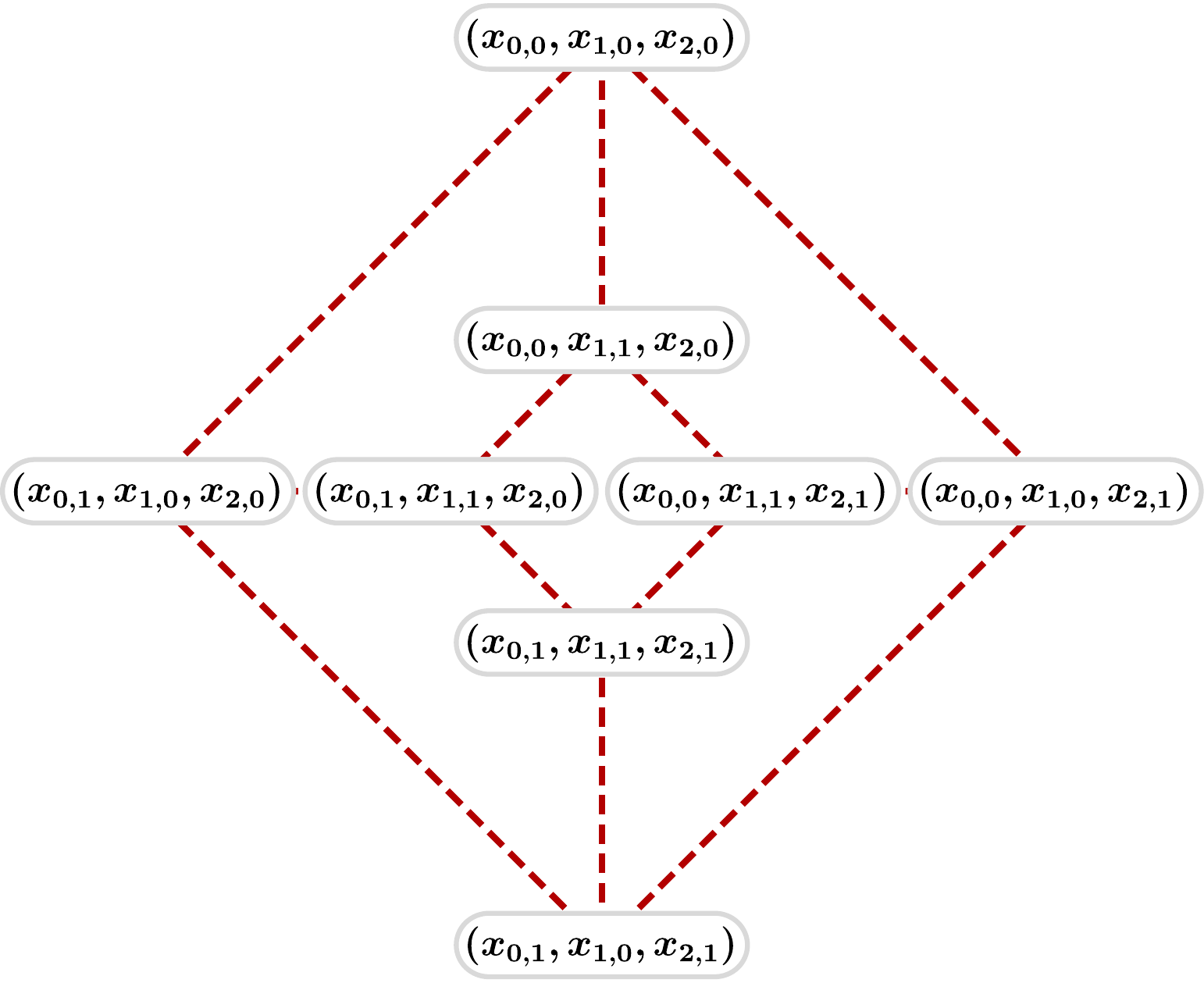
In the context of a quantum search over the discretised solution space of a CMOP, the hypercube has the desirable property of (at least approximate) preservation of the solution space structure, as grids in one, two, and three dimensions can be embedded in a hypercube [Ost87]. Examples of the grid embedding induced by \(\hat{U}_{W\text{-QAOA}}\) are shown in Fig. hypercube-mixing-structure. Also, a hypercube graph has a diameter of \(M\) and \(M\) disjoint paths between any two vertices [Ost87], so the distance between any two \(\bm{x}_k\) is exponentially smaller than \(K\).
|
|
Examples of the coupling produced on \(\bm{x}_k\) by \(\hat{U}_{W\text{-QAOA}}\) with a hypercube \(\hat{W}\) are shown for a solution space of size \(K=8\) in \(D=2\) and \(D=3\), respectively. The dashed red line indicates the grid embedding, which in this case is approximate for \(D=2\) and exact for \(D=3\).
QOWE
The Quantum Optimisation with Wavepacket Evolution (QOWE) algorithm is based on the approach to continuous-variable optimisation described in [VABK19] which, using continuous quantum variables, consists of the propagation of an initial Gaussian wavepacket under a phase-shift followed by the mixing unitary
where \(\hat{p}_d\) is the momentum operator conjugate to the continuous coordinate \(\hat{x}_d\). This choice is inspired by considering the quantum simulation of a particle evolving under the potential \(f(\bm{x})\).
Here we examine a discretised form of this algorithm, with the problem solution space encoded in \(\ket{k}\). The state is initialised to a discretised Gaussian wavepacket,
where \(x_{k}^{(d)}\) is the \(d^{th}\) component of \(\bm{x}_k\), \(\mu_d\) and \(\sigma_d\) are the centre and width of the wavepacket in each dimension, and \(A\) is a normalising constant. Discretising the mixing unitary requires a discrete form of the continuous momentum operator. For our implementation of QOWE, we construct a discrete analogue of the continuous-variable relationship \(\hat{p}_d = \mathcal{F}^{-1} \hat{x}_d \mathcal{F}\) (in each dimension), where \(\mathcal{F}\) is the continuous Fourier transform. The continuous Fourier transform along a single dimension can be approximated on the discretised grid as
where \(\text{DFT}\) is the centred discrete Fourier transform, and \(\kappa_{d,n_d} = \kappa_{d,0} + n_d \Delta \kappa_d\) is a momentum-space grid point, with \(\Delta \kappa_d = \frac{2\pi}{N \Delta x_d}\), \(\kappa_{d,0} = \Delta \kappa_d ( -N + 1 + \lfloor \frac{N-1}{2} \rfloor )\), and \(n_d = 0, \dots, N-1\). The corresponding Fourier transform over the entire discretised solution space is then \(F := \otimes_{d=0}^{D-1} F_d\), and the mixing unitary is
where \(\hat{W}_{\kappa}\) is the diagonal operator,
and where \(\bm{\kappa}_k = (\kappa_{0,n_0}, \dots, \kappa_{D-1,n_{D-1}})\) is a momentum space grid point with a similar indexing to \(\bm{x}_k\).
Applying the phase-shift unitary followed by the first Fourier transform in (29) and computational basis measurement is related to Jordan’s algorithm for gradient computation [Jor05]. Here, the gradient information is used coherently by following the first Fourier transform by the remaining two unitaries in (29), instead of performing a measurement.
QMOA
The Quantum Multivariable Optimisation Algorithm (QMOA) mixer is taken to be a unitary of separable CTQWs,
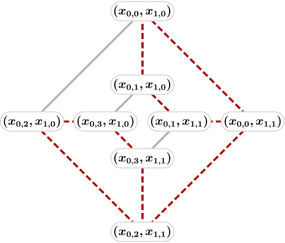
where \(\bm{t} = (t_0,...t_{D-1})\) with \(t_d \geq 0\) and \(\hat{C}_d\) is the adjacency matrix of an undirected graph (see (23)) connecting vertices along the dimension \(d\). The discretisation of the QOWE mixer is of a similar form if the generator of (29) is interpreted as a composite of complete graphs with complex-valued \(w_{kk'}\). In QMOA, we only consider cases where \(w_{kk'} \in \{ 0, 1 \}\). With \(\hat{C}_d\) as a cycle graph, \(\hat{W}\) is equivalent to a finite difference approximation of the Laplacian (i.e., a different discretisation of (27)). However, we consider more general graphs that do not correspond to different discretisations of (27), but do separate into independent quantum walks in each dimension. The case where each \(\hat{C}_d\) is a complete graph is depicted in Fig. QMOA-mixing-structure for a two-dimensional \(4 \times 4\) grid.
Under the condition that \(\hat{C}_d\) is circulant, and therefore diagonalised by the coefficient matrix of the discrete Fourier transform, (31) is efficiently realisable as
where \(\text{DFT}\) denotes the discrete Fourier transform and,
is constructed using the closed form solution for the eigenvalues \(\Lambda_{d,n_d}\) of \(\hat{C}_d\). We note that of the graphs introduced for the QAOA, the complete graph is circulant, while the hypercube graph is non-circulant. Altogether, the QMOA ansatz unitary \(\hat{U}_\text{QMOA}\) has a \(\mathcal{O}\left(\text{polylog} \, K\right)\) gate complexity resulting from \(D\) instances of the quantum Fourier transform [HH00].
For complete graphs \(\hat{C}_d\), the mixing unitary can be written as,
In each dimension, the operator \(\exp(-i t \hat{C}_d)\) applies an unbiased coupling between all points within each line parallel to coordinate axis \(d\). The amplitude of a point then evolves according to the average amplitude along the corresponding line, analogous to (25). Combining the walks in each dimension, along with the phase-shift, \(\hat{U}_\text{QMOA}(t, \gamma)=\hat{U}_{W\text{-QMOA}}(t)\hat{U}_Q(\gamma)\) causes the amplitude of a point to evolve according to the locally phase-encoded \(f_k\) relative to averages of phase-shifted amplitudes in the various subspaces containing the point. For example, in Fig. QMOA-mixing-structure the coordinate subspaces of \(\ket{k=13}\) are the row of points containing \(x_{0,3}\) and the column of points containing \(x_{1,1}\). By averaging phase-shifted amplitudes among these subspaces, rather than simply over the entire solution space as in (24), as well as using different walk times \(t_d\) in each dimension, \(\hat{U}_{W\text{-QWOA}}\) can break degeneracies resulting from contours in \(f\) that are non-parallel to the coordinate axes. More generally, the evolution of amplitudes at any two \(\ket{k}\) will respond similarly to variations in \(t_d\) and \(\gamma\) only if there is similarity in their locally encoded \(f_k\) and the averages of the phase-encoded \(f_k\) in their respective subspaces, which is likely to occur only when there is a high degree of symmetry in \(f\). Furthermore, as the minima of a continuous \(f\) are stationary points, every line passing through (or near) a minimum will contain multiple \(\bm{x}_k\) with \(f_k\) close to the minimum value (provided the discretisation is sufficiently dense). Consequently, the separable CTQWs have the potential to mutually re-enforce convergence to subspaces that contain multiple high-quality solutions.
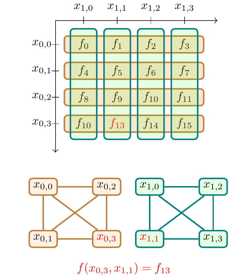
Fig. 4 Overview of the QMOA for an arbitrary \(f\) in \(D=2\) discretised over a grid of 16 points. The horizontal and vertical outlines denote the hyperplanes of constant coordinates. The bottom two graphs in (a) illustrate the coupling between these hyperplanes in \(\hat{U}_{W\text{-QMOA}}\) with a complete graph in each dimension.